Fit an accelerated life model and extrapolate to use conditions
Before you start: Failure times gathered at two or more stress levels (three is better), with the stress recorded per unit.
You can't wait ten years to find out whether something lasts ten years. So you run it hot, or at elevated voltage, or under heavier load, until it fails on a timescale you can actually observe — and then work backwards to what it would have done at normal conditions.
That's accelerated life testing, and it lives in its own section of Reliafy because the workflow genuinely differs from an ordinary life fit. A normal fit describes failures at one condition. ALT fits failures across several stress levels plus a relationship tying life to stress, which is what lets it extrapolate to a condition you never tested.
What your data needs
One row per unit, with the failure time and the stress that unit was running at:
hours,temp_K,censored
1350,333,0
950,353,0
620,373,0
Two stress levels is the bare minimum; three or more is much better, because with only two you're fitting a line through two points and have no way of noticing it's the wrong line. Censored units are fine and common — tests get stopped before everything fails.
You can also model two stresses at once (temperature and voltage, temperature and humidity), which needs a crossed design so the two aren't confounded.
The assumption underneath all of this: raising the stress must accelerate the same failure mechanism, not introduce a new one. Bake a component past the point where a different mode kicks in and you're no longer learning anything about field failures. Keep the stresses within the range where the physics is the same.
Choosing the model
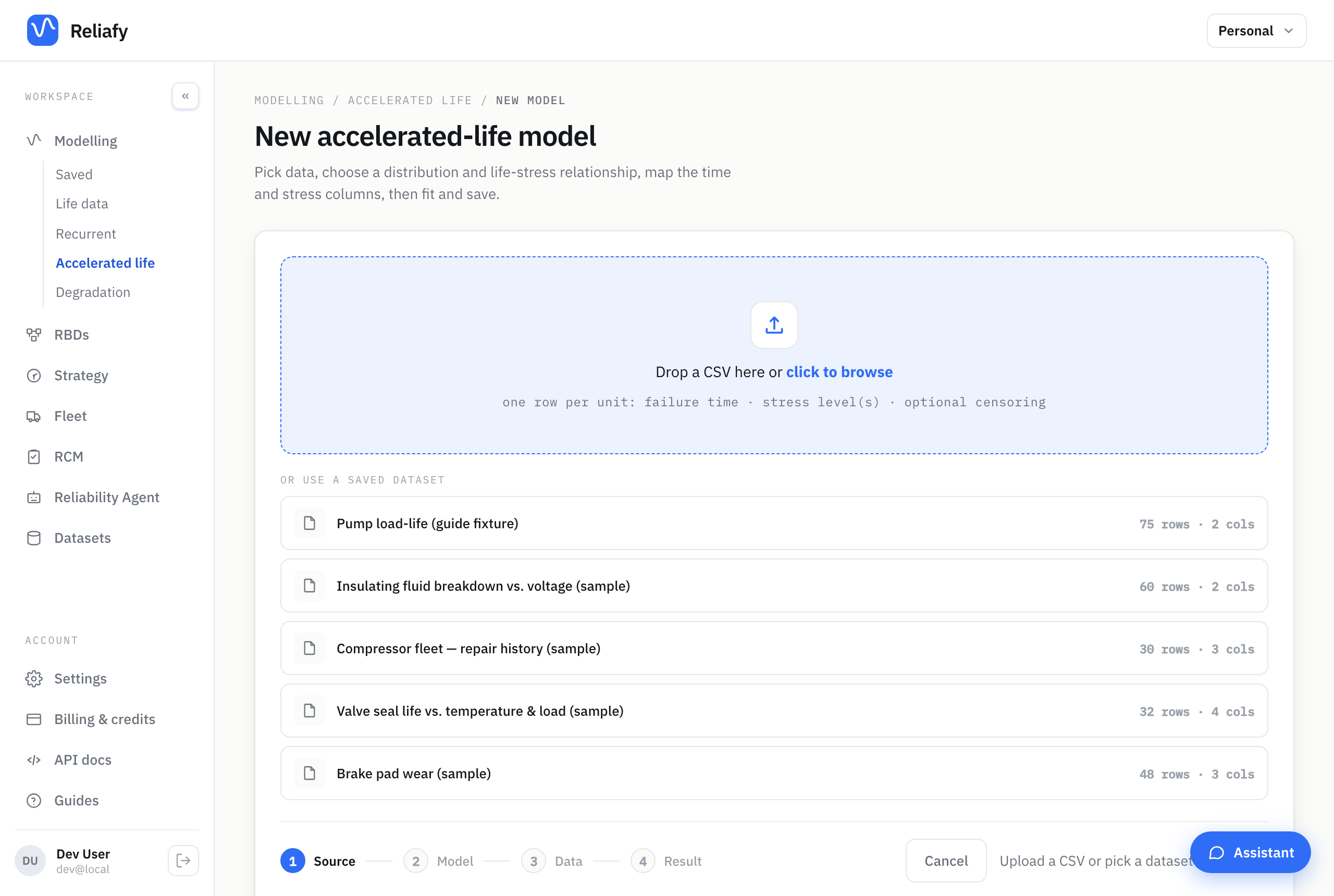
Go to Modelling → Accelerated life → New model. The flow asks for the model before the data, which is deliberate — the life-stress relationship determines how many stress columns you'll be mapping.
You pick two things:
- A life distribution — Weibull, lognormal, normal, exponential or gamma. This describes the scatter in failure times at any fixed stress.
- A life-stress relationship — how the characteristic life shifts as stress changes.
Match the relationship to the physics:
- Arrhenius for thermal ageing. Use absolute temperature (kelvin) — this trips people up constantly, and using Celsius will give you a nonsense fit.
- Inverse power law for voltage, load, or pressure.
- Eyring as a physically-derived thermal alternative to Arrhenius.
- Linear for a simple straight-line trend of life with stress.
- Dual exponential (temp–humidity), Temperature–nonthermal or Dual power for two stresses together.
Then map your columns — the failure time, the stress column(s), and censoring if you have it — and fit.
Reading the fit
Two views matter, and they answer different questions.
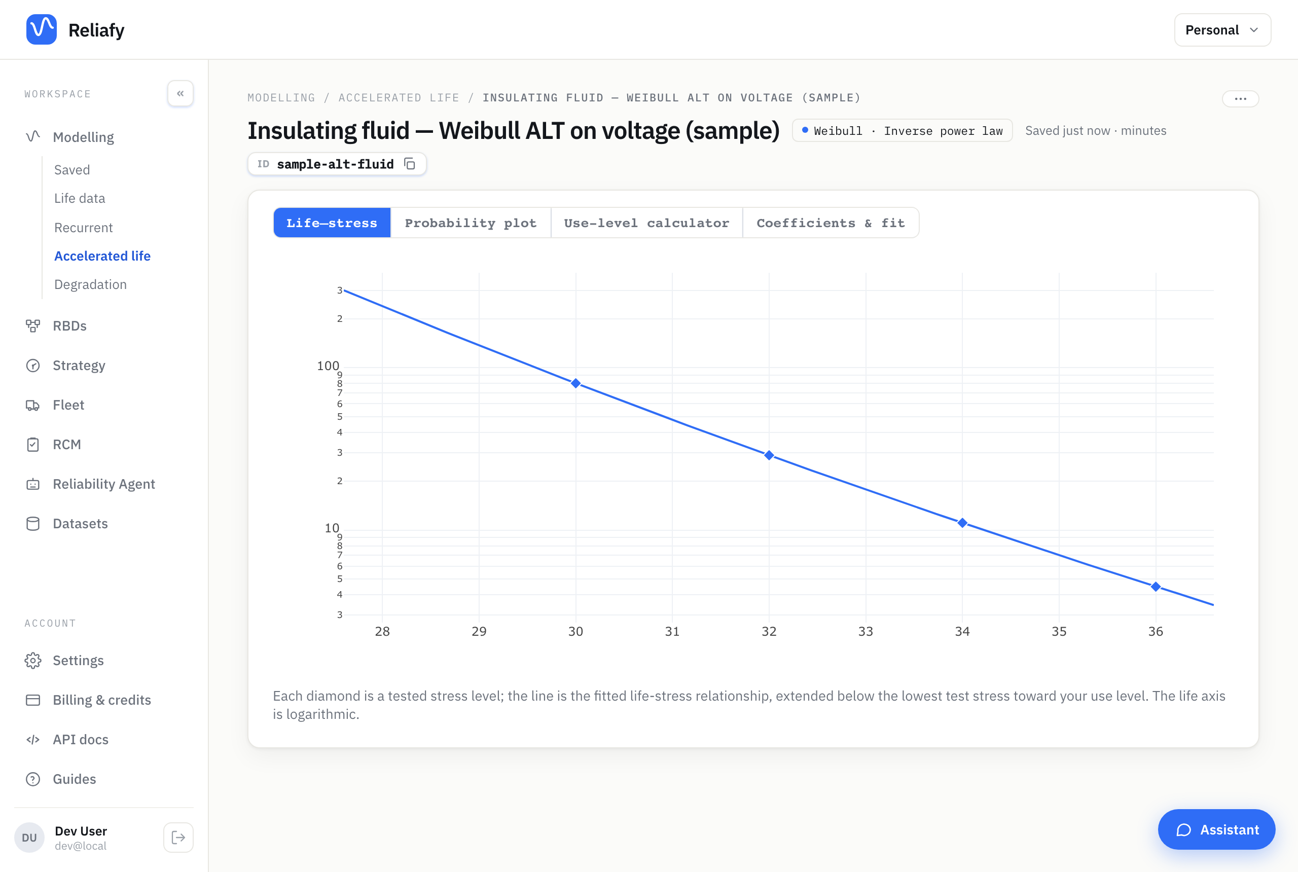
The life–stress plot is the ALT signature: characteristic life against stress, with each tested level marked and the fitted relationship drawn through them, extended below your lowest test stress toward use conditions. This is where you see whether the extrapolation is a short reach or a heroic one.
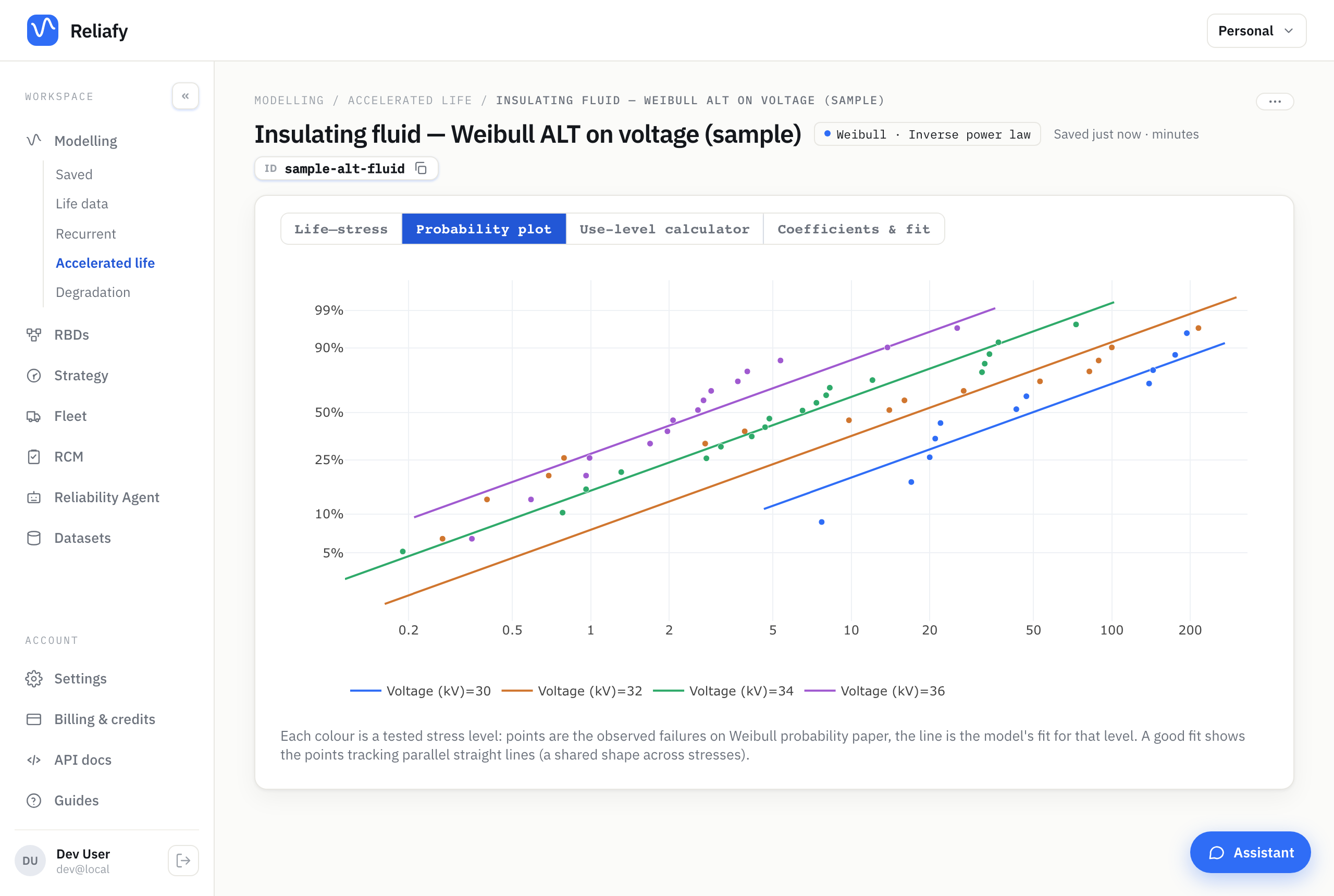
The probability plot is the honesty check. Each stress level's failures are drawn on the distribution's probability paper. A trustworthy fit shows the levels as parallel straight lines — parallel because the shape parameter is shared across stresses, straight because the distribution is right. If they fan out or curve, the shape isn't really constant across stress, and the extrapolation is resting on an assumption your data doesn't support. Better to find that out here than in the field.
Extrapolating to use level
Save the model and open the use-level calculator. Enter the stress your equipment actually runs at — below your tested range, which is the whole point — and you get the extrapolated reliability curve, the characteristic life, mean life, and B-lives at that condition.
Give it a reference stress as well and you get the acceleration factor: the ratio of use life to test life. That's the number that makes test planning concrete. At AF = 100, one hour on the bench stands for a hundred hours in service, so demonstrating a 10,000-hour field life means surviving about 100 hours on test.
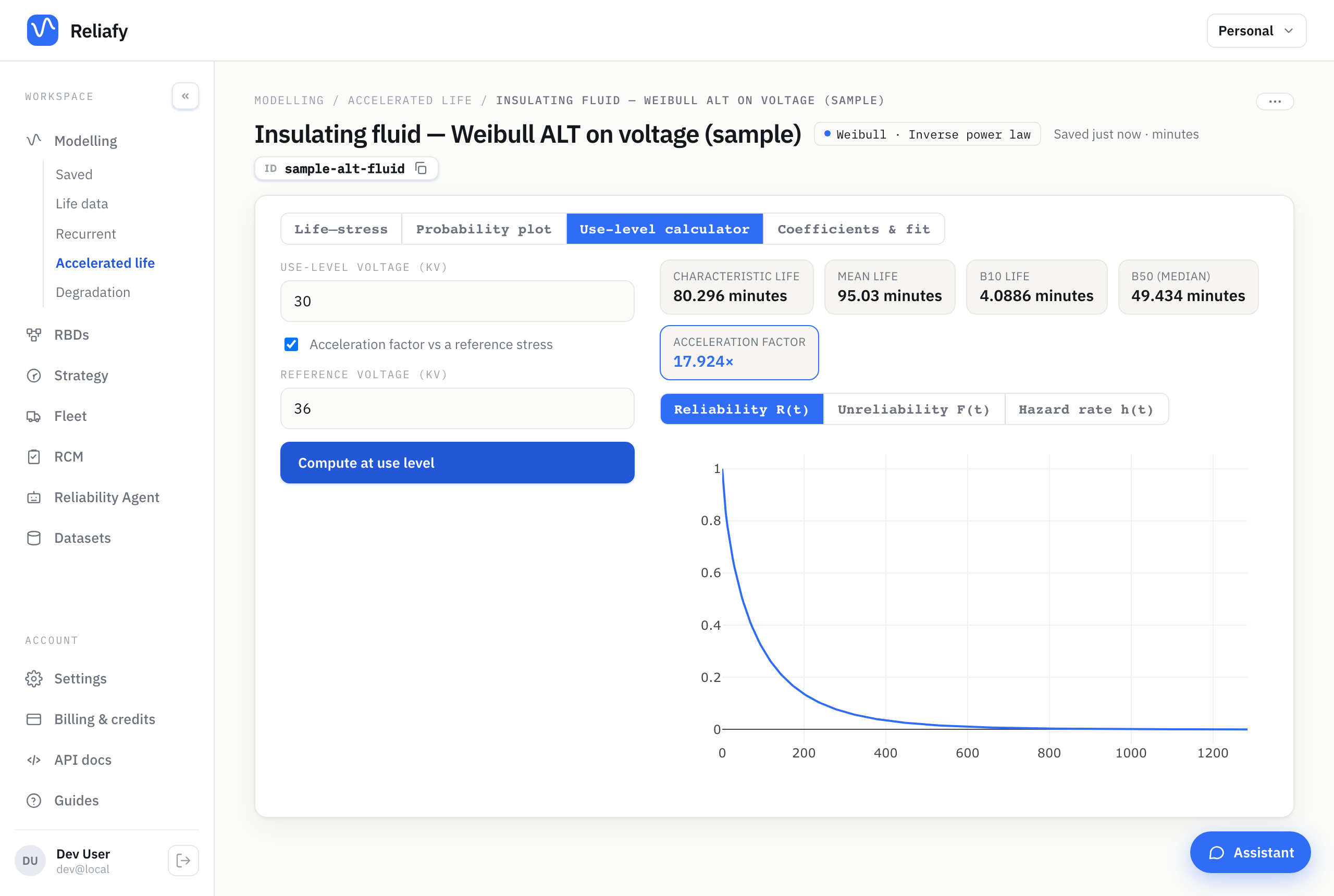
Treat the acceleration factor as a sanity check too. If it comes out implausibly large, you're either extrapolating much further than the data supports or you've fitted the wrong relationship.
Plan the next accelerated test
A fit also tells you how to run the next test better. Under the results of a saved model, Plan the next accelerated test from this fit opens Strategy → Test planning on the Accelerated test tab, with the fit's life-stress model, its coefficients, its shape and units already filled in, and the highest stress you tested as the Highest test stress.
The trade-off it settles is simple. A higher stress gives failures quickly, but the further the test stress is from normal use, the further the answer is extrapolated, and the less precise it is. The plan picks the lowest test stress and splits the units between the stresses so the life at use comes out as precisely as the test allows.
Give the Use stress and press Compute. For the sample insulating-fluid model (failures against voltage, in minutes), a use stress of 20 kV, 40 units and a 1,000-minute test give:
Test 34 at 23.6 kV, 6 at 36 kV, each for 1,000 minutes. Expect about 16.9 failures in all. The test estimates B10 at the use stress (20 kV: 2,504 minutes on these planning values) to within a factor of 2.79 at 90% confidence.
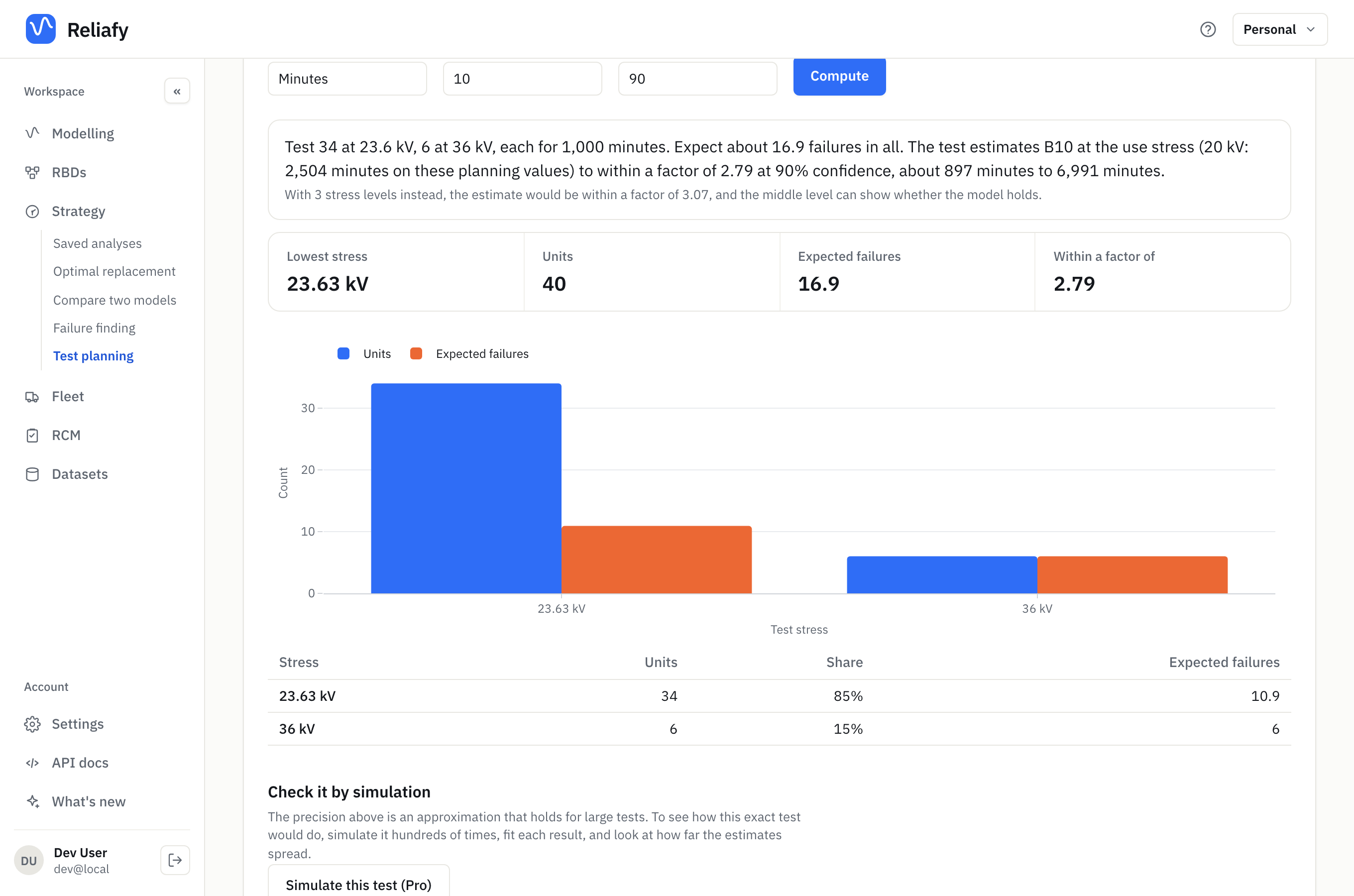
Most units go to the lower stress: it is closer to use, but fewer of its units fail, so it needs more of them. The highest stress needs only a few, because they fail quickly. Stress levels offers 3 or 4 levels instead of 2: a little less precise, but the middle level shows whether the life-stress model really holds. Check a test of my own works out what a test you have already designed would give.
Plans take one stress, a Weibull or lognormal distribution, and the Arrhenius, Eyring or inverse power law model. Without a fit, open the tab directly and type planning values from a similar part.
Where to go next
The relationships, the activation-energy interpretation, and a worked temperature example are in the Learn article on accelerated life testing.
The models come from SurPyval, an open-source Python library; its accelerated life documentation fits them in code.
If your interest is the opposite direction — what happens as surviving units get more stressed — see load-sharing, which uses the same kind of stress-life model in reverse.