Analyse repairable systems and reliability growth

Life-data analysis models time to a single failure — an item is born, it lives, it dies, and that's the end of its story. That's the wrong frame for a repairable system, which fails, gets fixed, goes back into service, and fails again. A compressor that's been repaired eleven times doesn't have "a life"; it has a history.

The questions change too. Not "how long will it last?" but: is it getting better or worse? How often will it fail next year? Are the repairs actually helping?

That's the recurrent-events section, and it's the honest home for MTBF on repairable equipment.

What your data looks like

Long format: one row per event, saying which system failed and when.

compressor,hours,test_end
CMP-1,1150,5000
CMP-1,2050,5000
CMP-2,1400,5000

The key columns are i (the system identifier — this is what groups events into per-machine histories) and x (the event time, measured from that system's start, not a calendar date).

You should also give each system's observation window — how long you watched it, whether or not it failed again — mapped to tr. Without it the analysis can't tell the difference between a machine that stopped failing and a machine you stopped watching, and it will quietly conclude your fleet is improving.

Fitting

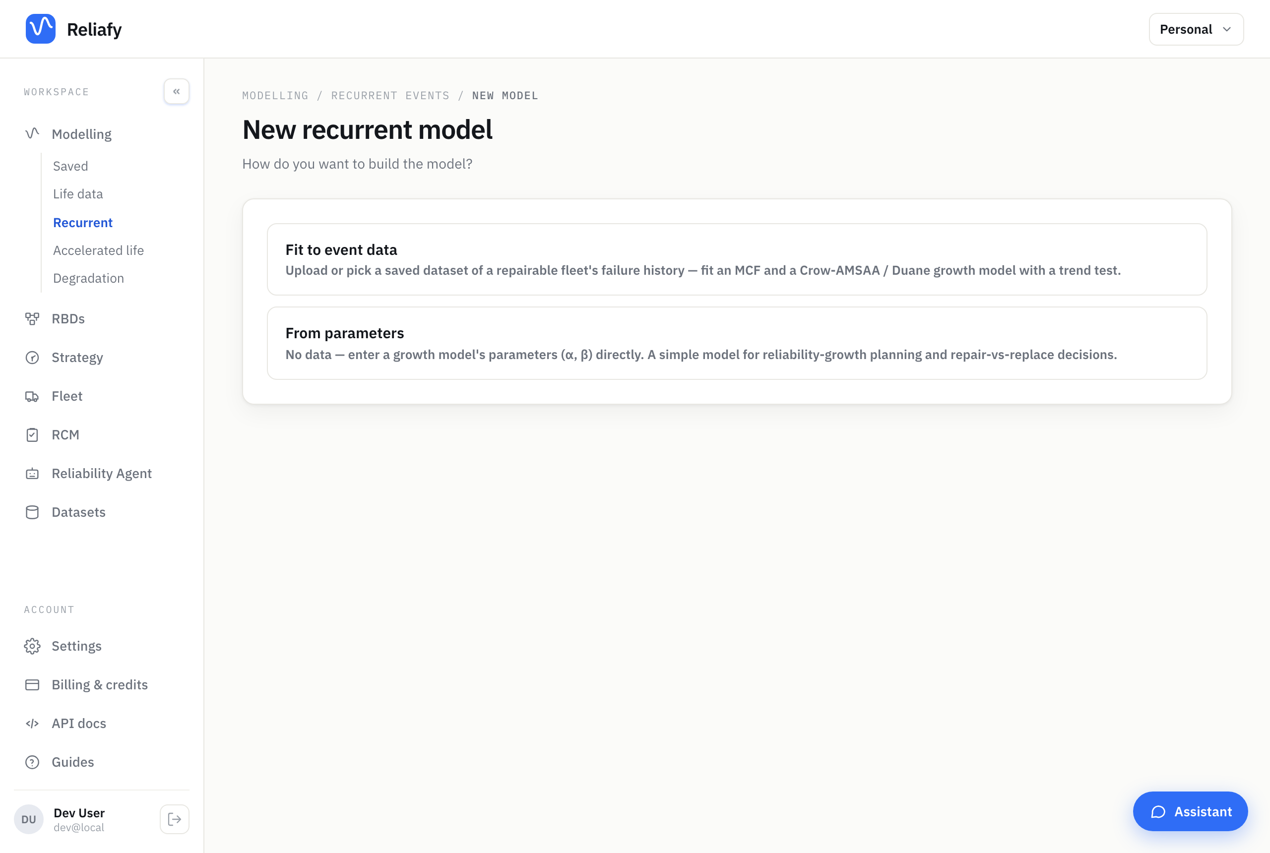
Go to Modelling → Recurrent events → New model, pick your data, map the columns, and choose a model:

• Crow-AMSAA (NHPP) — the standard reliability-growth model, and the right default.
• Duane — the classic log-log formulation of the same idea.
• Homogeneous Poisson (HPP) — a constant failure rate with no trend. Useful mainly as a null model to compare against.

You can also build one from parameters if you already know α and β and just want the calculator — handy for growth planning before you have data.

Reading the result

The mean cumulative function (MCF) plot is the heart of it: cumulative failures against time, with the observed step function and the fitted curve. Its shape is the finding. Curving upward means failures are accelerating; flattening means they're slowing; a straight line means a steady rate.

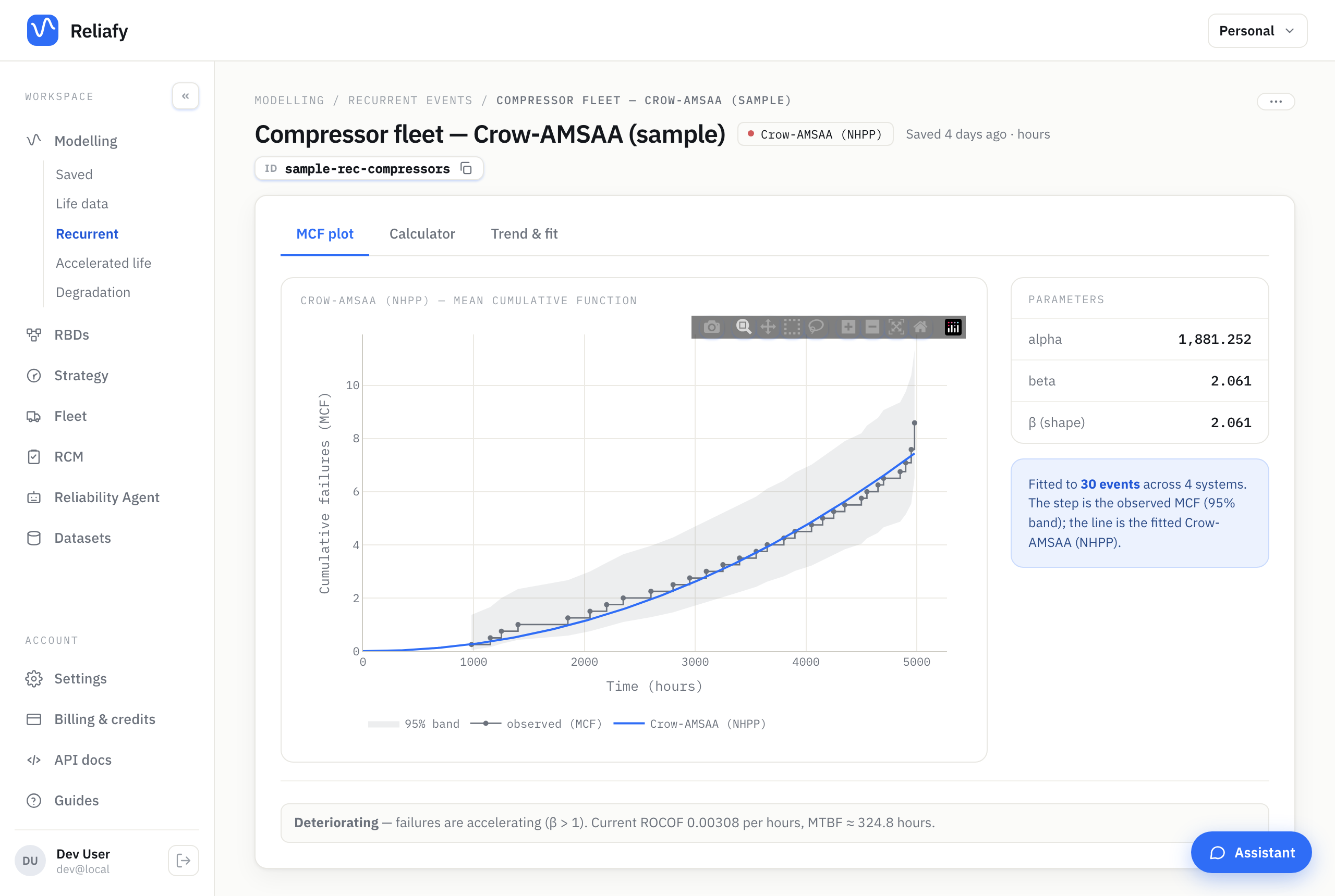
The number that formalises this is β:

• β < 1 — improving. Failures are getting rarer. Reliability growth is real.
• β ≈ 1 — stable. A constant rate; repairs are restoring the system to roughly where it was.
• β > 1 — deteriorating. Failures are accelerating. The system is wearing out faster than repairs restore it, and there's usually a decision waiting at the end of that trend.

Reliafy states the verdict in words alongside the number, plus the current ROCOF (rate of occurrence of failures) and the instantaneous MTBF — the honest MTBF for a repairable system, which is a current rate rather than a lifetime average.

A trend test (Laplace) tells you whether the trend is statistically significant or whether you're reading noise. Worth checking before you take a deteriorating verdict to a capital-expenditure meeting.

The calculator

The calculator answers the planning questions directly: expected cumulative failures by a future time, the failure rate at a given point, and how many failures to expect in a specific window — which is the number that sizes a spares order or a maintenance budget.

Where to go next

If the same equipment also has a wear-out story at the component level, fit those as ordinary life models — the two views answer different questions and are complementary, not competing.

If you're deciding whether to keep repairing or replace outright, a recurrent model built from parameters feeds that comparison directly.